3D Test problems
MARIN
The problem consists of a 1m x 1m x 0.55m column of water, initially at rest, that collapses under the action of gravity and impacts a stationary object. The computational domain is a rectangular box with dimensions 3.22m x 1m x 1m. The object has dimensions 0.161m x 0.161m x 0.403m and is placed at the back end of the tank. The top of the domain is closed. For more details, see runfiles or references.
Preprocessing
No postprocessing is necessary for running this case. To be able to run hexahedral elements the single-purpose marinMesh mesh-generator needs to be compiled. This is part of the mprans default build sequence, so one can assume this utility is available.
The first lines of marin.py the discretion and formulation can be chosen by modifying the following lines.
| Parameter | Description |
|---|---|
| Refinement = 2 | Controls the global level or refinement e.g. 5 ==> 32x16x16 |
| spaceOrder = 1 / 2 | Choose linear or quadratic elements |
| useHex = True / False | Choose hexahedral or tetrahedral elements |
| useRBLES = 0.0 / 1.0 | Choose SUPG (0.0) or RBLES/VMS (1.0) for stabilizing the Navier-Stokes equations |
| useMetrics = 0.0 / 1.0 | Choose h-based (0.0) or metric based (1.0) numerical parameters |
Running
The benchmark can be run using the following command:
mpirun -n #NP parun marin_so.py -l 3 -v -O petsc.options -D lin_tet_3
where #NP stand for the number of processors. The final argument, which specifies the output directory, is optional. Or use one of the run.#HOST.pbs run files.
Postprocessing
For extracting pointwise pressure and waterheights at certain location in the tank 2 separate pvpython scripts are supplied in $PROTEUS_MPRANS/scripts. To be able to run the scripts pvpython needs to be installed. This is a special python shipped with paraview. Furthermore, the scripts assumed there is one master xmf file. This master xmf file can be generated by running the following command in the directory containing the xmf/h5 solution files.
$PROTEUS/proteusModule/scripts/gatherArchives.py -s #NP -f marin_p
This will generate a file marin_p_all#NP.xmf which can be used for extracting pressures and heights by running the following commands in the directory containing the xmf/h5 solution files.
$PROTEUS_MPRANS/scripts/marinExtractPressure.py -f marin_p_all#NP.xmf
$PROTEUS_MPRANS/scripts/marinExtractHeight.py   -f marin_p_all#NP.xmf
This will produce the files pressure.txt and height.txt that contain the pressure and height time series. The full experimental data is provided exp_full.dat, while exp_height.dat and exp_pres.dat only contain the relevant extracted form exp_full.dat.
For visualizing purposes it might be beneficial to repackage the xmf/h5 solution files. There are three distinct reasons/benefits to do this:
1. The script allows skipping time steps and only extracts variable deemed important, thereby greatly reducing the file size and hence the time to copy data form remote location.
2. In the resulting solution files every time step has a distinct solution file, which allows visualization of results while the simulation is still running.
3. The scripts also outputs VTK files which allows visualization with VisIt (and others).
Repackaging of the solution can be done by running the following commands in the directory containing the xmf/h5 solution files.
$PROTEUS_MPRANS/scripts/extractSolution.py -f ../marin_p -s #start -e #end -i #incr -n #NP
where #start end #end are the begin and end timestep number and #incr is a increment time step (aka stride) and #NP is again the number of processors.
For convenience all the postprocesing mentioned above are lumped in a simple script. This script can be run using following commands in the directory containing the xmf/h5 solution files.
postpro.sh
References
- K.Kleefsman, G. Fekken, A. Veldman, B. Iwanowski, B. Bucher (2005) A volume-of-fluid based simulation method for wave impact problems, Journal of Computational Physics, 206, 363-393
- C.E. Kees, I. Akkerman, M. W. Farthing and Y. Bazilevs (2011) A Conservative Level Set Method for Variable-Order Approximations and Unstructured Meshes, Journal of Computational Physics, 230-12, 3402-3414, doi:10.1016/j.jcp.2011.02.030
- I.Akkerman, Y. Bazilevs, C. E. Kees and M. W. Farthing (2011) Isogeometric Analysis of Free-Surface Flow Journal of Computational Physics, 230-11, 4137-4152, doi:10.1016/j.jcp.2010.11.044
Dambreak
The problem consists of a 0.146m x 0.146m x 0.292m column of water, initially at rest, that collapses under the action of gravity and impacts a stationary object. The computational domain is a rectangular box with dimensions 0.584m x 0.146m x 0.350m. The top of the domain is left open. For more details, see runfiles or references.
Preprocessing
No postprocessing is necessary for running this case. The first lines of dambreak.py the discretion and formulation can be chosen by modifying the following lines.
| Parameter | Description |
|---|---|
| Refinement = 2 | Controls the global level or refinement e.g. 5 ==> 32x16x16 |
| spaceOrder = 1 / 2 | Choose linear or quadratic elements |
| useHex = True / False | Choose hexahedral or tetrahedral elements |
| useRBLES = 0.0 / 1.0 | Choose SUPG (0.0) or RBLES/VMS (1.0) for stabilizing the Navier-Stokes equations |
| useMetrics = 0.0 / 1.0 | Choose h-based (0.0) or metric based (1.0) numerical parameters |
Running
The benchmark can be run using the following command:
mpirun -n #NP parun dambreak_so.py -l 3 -v -O petsc.options -D lin_tet_3
where #NP stand for the number of processors. The final argument, which specifies the output directory, is optional. Or use one of the run.#HOST.pbs run files.
Postprocessing
For extracting column heights and width a separate pvpython scripts are supplied in $PROTEUS_MPRANS/scripts. To be able to run the scripts pvpython needs to be installed. This is a special python shipped with paraview. Furthermore, the scripts assumed there is one master xmf file. This master xmf file can be generated by running the following command in the directory containing the xmf/h5 solution files.
$PROTEUS/proteusModule/scripts/gatherArchives.py -s #NP -f dambreak_p
This will generate a file dambreak_p_all#NP.xmf which can be used for extracting column heights and width by running the following commands in the directory containing the xmf/h5 solution files.
$PROTEUS_MPRANS/scripts/dambreakExtractHeightAndWidth.py -f dambreak_p_all#NP.xmf
This will produce the file height.txt that contain the height and width time series. The experimental data is provided by the file sakamoto_exp.dat
For visualizing purposes it might be beneficial to repackage the xmf/h5 solution files. There are three distinct reasons/benefits to do this:
- The script allows skipping time steps and only extracts variable deemed important, thereby greatly reducing the file size and hence the time to copy data form remote location.
- In the resulting solution files every time step has a distinct solution file, which allows visualization of results while the simulation is still running.
- The scripts also outputs VTK files which allows visualization with VisIt (and others).
Repackaging of the solution can be done by running the following commands in the directory containing the xmf/h5 solution files.
$PROTEUS_MPRANS/scripts/extractSolution.py -f ../dambreak_p -s #start -e #end -i #incr -n #NP
where #start end #end are the begin and end timestep number and #incr is a increment time step (aka stride) and #NP is again the number of processors.
For convenience all the postprocesing mentioned above are lumped in a simple script. This script can be run using following commands in the directory containing the xmf/h5 solution files.
postpro.sh
References
- S.Koshizuka, H. Tamako, Y. Oka (1995) A particle method for incompressible viscous flow with fluid fragmentation” Computational Fluid Mechanics Journal, 113, 134-147
- R.Elias, A. Coutinho (2007) Stabilized edge-based finite element simulation of free-surface flows, International Journal of Numerical Methods in Fluids 54, 965-993
- C.E. Kees, I. Akkerman, M. W. Farthing and Y. Bazilevs (2011) A Conservative Level Set Method for Variable-Order Approximations and Unstructured Meshes” Journal of Computational Physics, 230-12, 3402-3414, doi:10.1016/j.jcp.2011.02.030
Dambreak flow with tall obstacle - Gomez-Gesteira and Dalrymple (2004)
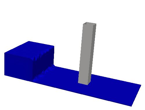
The problem consists of a 0.4m x 0.3m x 0.61 (dx x dz x dy) column of water, initially at rest. Under the action of gravity, the water column interacts with an obstacle and collapses to a wall. The computational domain is a 3D rectangular box with dimensions 1.6m long x 0.61m x 0.75m high. The obstacle has dimensions 0.12m x 0.12m, it is placed on the tank’ s bottom and reaches the top of the doamin. The top of the domain is left open, when the rest of the boundary patches act as no slio walls. In the following figure, a sketch of the dambreak initial conditions is shown.
This case tests the ability of PROTEUS to simulate the free-surface evolution and forces / pressures on structures. The results of the simulations can be compared with the data in the following references. For more details, see runfiles or references.
References
- Gómez-Gesteira, M. and R.A. Dalrymple, “Using a 3D SPH Method for Wave Impact on a Tall Structure, J. Waterway, Port, Coastal, Ocean Engineering, 130(2), 63-69, 2004.
Wave diffraction - Penny and Price (1952)
Wave diffraction presents a boundary behaviour of waves associated with the bending of their path. Wave diffraction involves a change in direction of the wave propagation as they pass through an opening or around a barrier. The waves are, then, seen to pass around the barrier into regions behind it and disturb the water behind it. The present benchmark case represents the case of wave diffraction caused by a semi-infinite breakwater. Analytical solutions for this type of diffraction are presented in Penny and Price (1952) and can be used for comparisons of the corresponding results of PROTEUS. The case is simulated using a 3D rectangular numerical domain with height of 1.5 m, a length, L, of 25.0 m and width, b, of 30.0 m. The breakwater is represented as a vertical thin solid wall with length, b1, equal to 10.0 m. The mean water depth within the domain is equal to 1.0 m. within the left boundary and the generation/absorption zone, non-linear waves are generated with a height of 0.10 m, a period of 1.94 s and a length of 5.0 m. Also, the waves are absorbed within the implemented absorption zone. For the determination of the flux parameters, the Fenton Fourier Transformation theory is used (Fenton, 1988). Atmospheric conditions have been assigned to the top boundary of the domain and the bottom boundary, the surfaces of the breakwater, the front and the back boundaries act as free-slip walls.
A sketch of the plan of the 3D domain of the present case is given in the following figure.
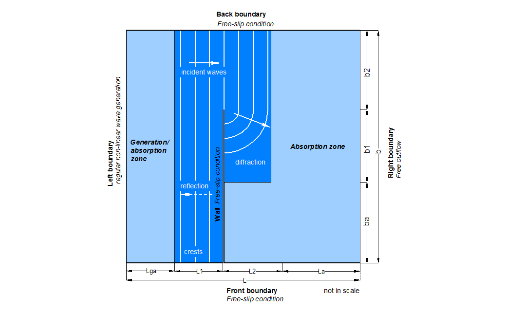
where,
- Lga=1 wavelength (=5.0m), the length of the Generation/absorption zone
- L1=L2=1 wavelength (=5.0m)
- La=2 wavelengths (=10.0m), the length of the Absorption zone in the x direction
- ba=2 wavelengths (=10.0m), the length of the Absorption zone in the y direction
- b1=b2=2 wavelengths (=10.0m)
This test case demonstrates the ability of PROTEUS to simulate the wave diffraction caused by a semi-infinite breakwater as well as the wave absorption within a 3D domain configuration.
References
- Penny WG and Price AT (1952) The diffraction theory of sea waves and the shelter afforded by breakwaters. Part I in u201cSome gravity wave problems in the motion of perfect liquidsu201d by Martin JC, Moyce WJ, Penny WG, Price AT and Thornhill CK, Philosophy Transaction of the Royal Society in London, A244, 236u2013253.
- Fenton JD (1988) The numerical solution of steady water wave problems. Computer and Geosciences, 14(3), 357-368.